CuTeDSL at Perplexity

At Perplexity, we use the in-house Runtime-Optimized Serving Engine (ROSE) to serve models ranging from embeddings to trillion-parameter LLMs. Sitting behind all APIs, including Sonar, Search, and Embeddings, our runtime was built to empower researchers to explore the most suitable models and architectures, while also quickly deploying the best candidates into production. To achieve this, we need to be able to implement, deploy, and optimize inference for state-of-the-art architectures at a rapid pace. In this blog post, we explore how CuTeDSL kernels integrated into our inference engine allow us to build the required GPU kernels to bring models up to peak performance on NVIDIA GPUs.
Inference at Perplexity AI
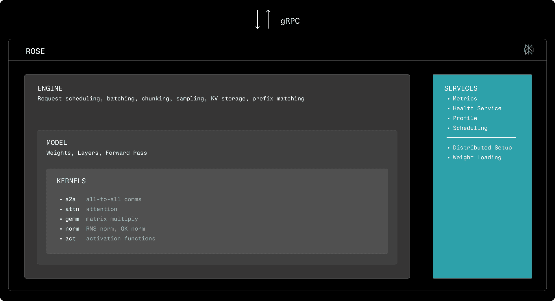
Custom models, built by various teams at Perplexity, are hosted in-house on NVIDIA Hopper and Blackwell GPUs using the ROSE inference engine built by the AI Inference team. ROSE was initially built to better serve customized Llama models for both language decoding and classification, with an interface compatible with the NVIDIA Triton Inference Server. Over time, it grew into a full-blown inference engine serving substantial LLMs, as well as ranking, classification, scoring, and other transformer-based models for a wide range of teams to power Perplexity’s products. The design goal of ROSE is to be simple: over time, effort is invested to reach peak performance, but the main priority is to adapt to the ever-evolving architectures and use cases for our models.
At a high level, ROSE consists of an engine which adapts a model to an interface clients can interact with. The engines are highly reusable, handling request scheduling and batching, and retrieving decoded tokens, embeddings, or scores from the underlying models. The initialization of devices, inter-process and inter-node communication channels, and weight loading are all handled by them. For LLMs, the engine is responsible for batching, chunking, sampling. It is also responsible for KV storage allocation, for both full and linear attention, as well as prefix matching. Embedding engines are simpler, as they only perform on-line batching. Execution is optimized such that the engine prepares the next round of work while the model is running on the accelerator in parallel.
ROSE exposes a rich collection of custom layers for modeling, wrapping GPU kernels built with CuTeDSL, Triton, CUDA, CUTLASS, and cuBLAS. For matrix multiplication and attention implementations, we primarily rely on NVIDIA kernels from CUTLASS and cuBLAS. The remainder of the pipeline, including embedding, norm, MoE, and activation kernels, are part of the kernel library of ROSE. To best support the hardware we run inference on, ROSE is equipped with its own inter-device communication primitives for MoE routing, dispatch, and combine. While the other kernels are relatively simple, they must be thoroughly specialized to achieve peak performance on all the different hidden dimensions and devices they run on. Additionally, we rely on compile-time specialization to accommodate all the knobs and tweaks of various models (weight bias vs. no weight bias for RMS norm, activation functions, etc.). Consequently, we decided to use DSLs to implement them: we initially built ROSE using Triton. However, we have since adopted CuTeDSL as the primary environment for GPU programming.
Why CuTeDSL?
From a mathematical perspective, inference kernels are usually unsophisticated. Consequently, when developing a kernel, the complexity generally does not lie in expressing what computation is to be done, but in how exactly the hardware should do it. To build the best kernels, we require a language that offers the right abstractions over the underlying hardware. The right language enables us to specify the high-level operations to perform the computation, aggressively specializing and optimizing them across all points in a wide configuration space.
CuTeDSL is a Python-based DSL for NVIDIA GPUs built on top of CuTe layout algebra and MLIR. It compiles just-in-time to highly optimized PTX, while retaining control over low-level hardware primitives. It aims to offer the same features and performance as CUTLASS C++, without the expensive compilation times that hinder development speed. Out of the languages we have surveyed or worked with (including CUDA, cuTile, TVM IR and Triton), we consider it to be the best fit for the development of our kernels.
Overall, while not as high-level and succinct as Triton or cuTile, we found that the CuTe Layout Algebra and its compositions (exposed via cute.Tensor) were reasonable substitutes. Additionally, CuTeDSL offers unrestricted access to hardware primitives, providing us with the level of control we require to achieve peak performance in all edge cases. With CUDA, opportunities for compile-time specialization were limited, as each additional parameter added an unreasonable cost to compilation times or complexity to the build system. In contrast, with a Just-In-Time Compiled DSL, we can specialize more aggressively without sacrificing iteration pace. Unlike TVM IR, which used CUDA as an intermediate step, we found the MLIR-based pipeline that lowered to PTX to be more robust and easier to debug than one that emitted CUDA as an intermediate step. Additionally, with the use of custom ops to wrap PTX instructions, we found that we could fully leverage all the features of the underlying hardware.
Developer experience
The bulk of the compilation cost of CUDA kernels is typically spent in the template expansion phase of kernels, as optimization and compilation from the PTX stage onwards can be completed in a matter of seconds. With many compile-time parameters, this stage of compilation can explode to multiple minutes for a non-trivial kernel. This bottleneck is accentuated by the fact that opportunities for parallel compilation arise only later, at the IR and PTX levels, with C++ template handling happening sequentially. While tricks exist to address this, by moving template instantiations to separate compilation units, they require significant tweaks to build systems and the use of unwieldy macros. In contrast, CuTeDSL kernels that are compiled Just-In-Time (JIT) do not require complex build rules and do not hinder compilation times, as the development cycle can be focused on a single point in the configuration space, while careful unit tests later can cover the entire design space of the kernel.
Even though JIT compilation moves costs from development-time to runtime, the overhead is more than acceptable. When a model is deployed, it activates only a few of the points from the entire configuration space, incurring second-scale overheads during the startup/warmup of the inference engine. In contrast, pre-compiling all configurations of a kernel could span multiple minutes. Additionally, overheads can be further mitigated by caching the JIT-compiled artifacts.
The heavy compilation cost of CUDA is accentuated by the difficulty of tracing the origin of errors when template-based dispatch and specialization is used, as is the case with CuTe and CUTLASS. With a DSL, errors can be pointed to the line of code that generated it, significantly easing debugging. Additionally, it is much simpler to map the generated code to the DSL statement that originated it via intermediate MLIR stages or relying on debugging information attached to the generated PTX. Thanks to these aspects of the DSL, we found ourselves much more productive when developing kernels.
Large configuration space
While kernels share many similarities across models, they must still be equipped with a range of configuration knobs that can have a performance impact. Relevant parameters include:
Hidden Dimension/Head Dimension/Number of Attention Heads
Input/Output data types
Quantization scheme
Compile-time constants (biases, activation functions, etc.)
Compile-time specialization is useful for both performance and debugging. Particularly in a pipelined processor, as is the case with GPUs, a nonexistent branch is better than an always-taken or never-taken branch. Additionally, compiling a kernel for a specific set of configuration knobs results in fewer PTX/SASS instructions, which are easier to analyze and debug when using cuda-gdb during an investigation.
For a given batch size and configuration, the expected traffic to DRAM and the number of arithmetic operations can be estimated. Subsequently, optimal decisions can be made on a case-by-case basis for optimal grid allocation, synchronization, and the use of certain hardware features. CuTeDSL allows us to define and re-use components for deep specialization without incurring an unacceptable compile-time overhead.
Prefill and Decode Specialization
Generally, the performance of inference kernels must be optimized for two separate use cases:
Prefill: small batch size (few chunks, sequences), many tokens per sequence. Throughput to be maximized for both embeddings and the input tokens of LLMs. Latency in the tens to hundreds of milliseconds.
Decode: small-to-large batch sizes, one (no speculative decoding) to a few tokens per sequence (draft-target speculation, multi-token prediction). Latency close to kernel launch latency.
For GEMM and attention, the prefill stage runs on a large number of tokens and performance is bound by the compute throughput of the device. Decoding involves the same operation on small batch sizes, with execution times dominated by the cost of loading the activations and weights from DRAM into the streaming multiprocessors and tensor cores, constrained by the memory bandwidth of the device instead. Even though the batch size or the overall number of tokens in a batch is a relatively clear indicator, the switchover threshold between prefill and decode is more subtle because the memory bandwidth is also determined by the hidden dimension of the model and the data type of the activation. Kernels are consequently split into prefill and decode implementations if algorithmic differences or grid/block assignments would advantage either of them.
The parameter which is universally different between prefill and decode kernels is the number of warps in a block (the number of threads, divided by the warp size of 32 threads per warp). It is desirable to make this parameter a compile-time constant, as it can aid in register allocation. In CUDA, this is typically done by specifying the number of threads via __launch_bounds__ and providing the number of warps as a template parameter:
The number of registers available to all threads in a block is a hardware constraint, 64K on Hopper and Blackwell. If the number of threads is known ahead of time, the compiler knows exactly how many registers it can assign to each thread and can succeed in compiling more aggressively optimized kernels. However, this comes at a compilation-time cost, as now the kernel has to be recompiled for different warp sizes. With CuTeDSL, this is no longer a problem, as we do not need to pay the cost of compilation for the entire configuration space upfront. The DSL also expects the block size to be a constant expression, implicitly performing the optimization implied by __latch_bounds__ in CUDA.
Besides making the number of warps a constant, it is desirable to vary it between prefill and decode. To fully utilize the memory bandwidth of a GPU, it is not sufficient to always assign a high number of warps per block, as full bandwidth can only be achieved by using as many of the available Streaming Multiprocessors (SMs). Consequently, for a given number of tokens and known data types and hidden dimensions, we first pick an ideal per-thread vector dimension (8 for bfloat16, 4 for float32) to ensure that the generated code uses the 128-bit load/store instructions (256-bit on Blackwell). Knowing the vector size, we can compute the number of warps required by the kernel. We first try to maximize the number of SMs: if there are less warps then SMs, a single warp per block is chosen. This is typically the decode variant of the kernel. If there are enough warps, we gradually increase the number of warps to 8, 16 or 32, benchmarking an upper bound after which we typically no longer see an improvement in performance.
While Triton performed some of these optimizations under the hood, we found that we can achieve similar results by carefully using CuTe layout algebra, without being constrained by the shortcomings of a high-level compiler. Particularly when sub-warp horizontal reductions are involved, we found that CuTeDSL offered us the fine-grained control required to generate optimal code.
Grid synchronization
In some situations, to distribute work across as many blocks as possible, cooperative_groups::this_grid().sync() can be used to synchronize all participating blocks. Restrictions apply: since a block cannot be de-scheduled from an SM once it starts execution, to guarantee forward progress, the number of blocks cannot exceed the number of SMs available on the device, to ensure that at any point all blocks can update and poll the global memory locations involved in synchronization. This restriction is enforced by cudaLaunchCooperativeKernel. The cost of a grid barrier is about 3us on Hopper, plus the cost of flushing all previous memory operations via an implicit memory barrier in some situations. Overall, this is comparable to the overhead of splitting a kernel into two launches, leading to a performance-sensitive design decision. Despite the fact that Programmatic Dependent Launch (PDL) can reduce launch overheads from Hopper onwards, for decode kernels, avoiding the overhead is worthwhile.
If one of the workloads requires more blocks than the number of SMs, the kernel should be split, relying on the implicit barrier of kernel launches. This is primarily the case for prefill. If the number of blocks which are ideal for all workloads fits in the grid, a grid barrier is preferred, as is the case with the decode kernels operating on a smaller number of tokens.
In CuTeDSL, these decisions can be made in the host-side launch code and the kernels can be composed and interleaved with grid barriers as necessary, as illustrated by the example below. With such a hybrid strategy, decode kernels can be optimized to reach minimal latencies and prefill ones can be optimized for maximal throughput. Unlike CUDA-based solutions, this logic can be defined more succinctly and with less compilation-time overhead.
In the case of our MoE all-to-all kernels, as detailed below, having the flexibility to build kernels with or without grid barriers and optimize them at compilation time helped us achieve substantial performance gains through CuTeDSL.
CuTeDSL Kernels
QK Norm
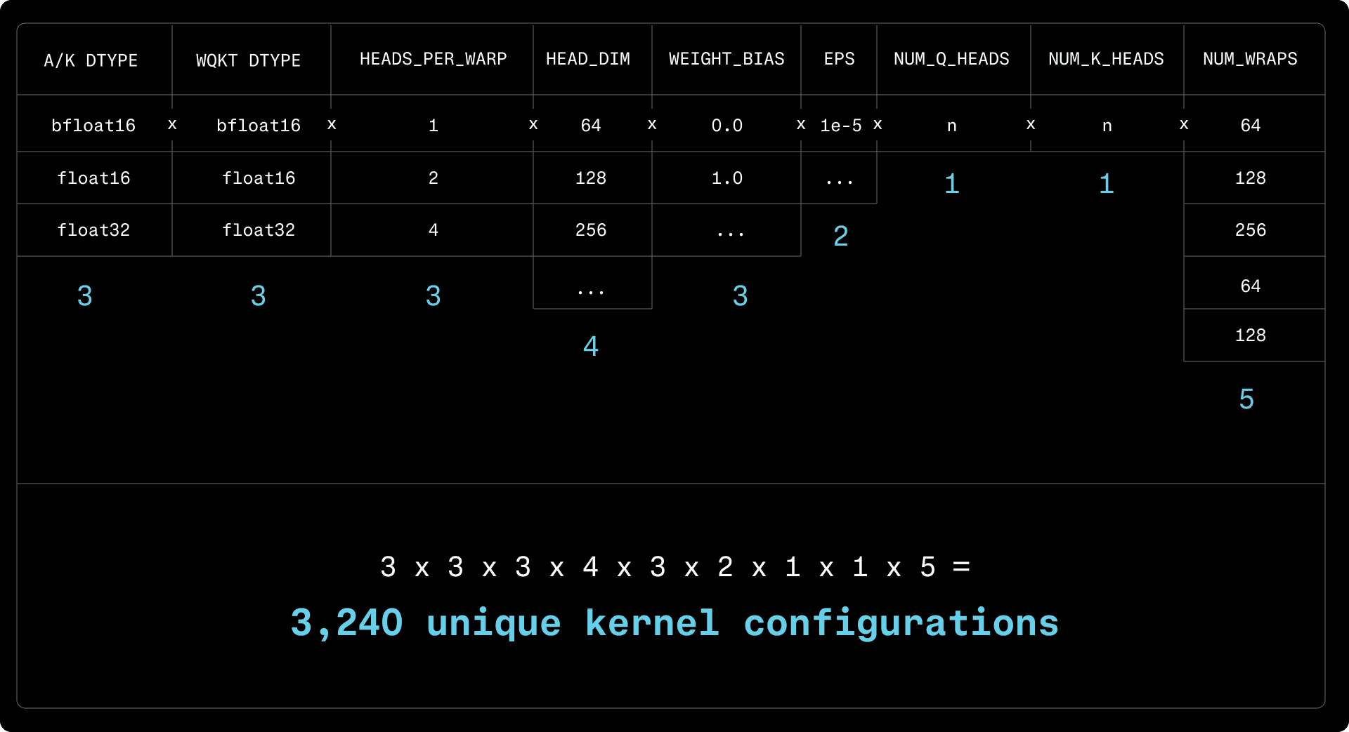
The first kernel we built in CuTeDSL was a specialized RMS norm kernel, optimized for small dimensions. QK norm, used in the self-attention layer of the recent Qwen models, is applied on a per-head basis, on 64, 128 or 256 elements. Unlike regular RMS norm, which operates on hidden dimensions exceeding thousands, requiring a horizontal reduction through both shared memory and registers, QK norm needs reduction only across warps, with the possibility of squeezing multiple heads into a single warp. This became a use case where we could aggressively optimize at compile time to find the best token-to-warp assignments for all head dimensions and data types.
RMS norm is a fairly straightforward operation, although it requires a horizontal sum to compute the squared norm of a vector:
Since attention heads are typically small and per-thread operations are heavily vectorized, a single warp can compute the square norm. In order to maximize memory bandwidth, each thread should process 128 bits of input, which translates to 8 bfloat16 values. Consequently, a half-warp is sufficient to process a head, and the squared norm can be determined using a horizontal reduction performed by shuffle_sync_bfly. Starting from the head dimension and the data type, we can determine the number of heads per warp and specify the arguments and the number of reduction rounds at the time of compilation.
We can then build a specialized kernel with relatively few lines of code, relying on automatically vectorized loads/stores and using lower-level architecture-specific operations for the warp reduction. The kernel determines which head (Q or K) to work on and identifies the corresponding weights to apply. It loads an entire vector from the head and first sums up locally. Subsequently, based on the number of threads per head, the squared norm is computed. Finally, the RMS norm, automatically vectorized, is determined and written back to memory. Model-specific parameters, such as WEIGHT_BIAS and EPS, are constant-folded.
Compared to a regular RMS norm kernel, this specialized variant delivers 2-3x better throughput and latency for both prefill and decode.
Mixture-of-Experts Dispatch/Combine
MoE dispatch and combine shuffle input tokens to the experts they are routed to, performing a weighted accumulation after MoE GEMM kernels perform the relevant matrix multiplications. Performance is of particular interest, as various products rely on MoE models of various sizes. Based on the deployment types, we distinguish different kernels to optimize:
TP=1: Local kernel for a single GPU. Dispatch shuffles tokens to the relevant experts and combine accumulates them. Used primarily for Qwen3 30B deployments on H100.
DP=1, TP ≠ 1: Tensor-parallel, singlenode kernel. The input is replicated, dispatch selects the tokens for the current rank, and combine accumulates them across all ranks. Accumulation across either NVLink or NVLS. Used for large prefillers.
DP ≠ 1, NVLink: Data-parallel kernel with optional tensor parallelism. Each rank sends tokens to each other rank hosting specific experts. Routing information is aggregated, tokens are transferred across NVIDIA NVLink. Used for data-parallel H200 or GB200 deployments.
DP ≠ 1, InfiniBand: Peer-to-Peer data-parallel and tensor-parallel kernel operating across both NVLink and NVIDIA Quantum InfiniBand. Used for multi-node Hopper deployments.
Local
The local kernel counts the number of tokens assigned to each expert based on the routing table and assigns a unique index to each token within the list of tokens belonging to each expert. After the routing step, the tokens are copied into optionally padded buffers to be passed on to an MoE GEMM kernel. Using the token locations, the combine kernel then performs an accumulation in registers, writing the final tokens into an output buffer.
The dispatch phase varies between prefill and decode: for few tokens, there is little routing information to read out, so we process it in a single block and signal the remainder of the grid, with individual blocks copying chunks of tokens. Token assignment is determined by atomically incrementing counters in shared memory. Since prefill must process more routing information, routing is split across multiple blocks in a separate kernel. Indices are first assigned locally using counters in shared memory and are then aggregated across all blocks in global memory to determine the position of each token. The grid of this kernel is clamped to the number of SMs in order to be able to use grid-wise barriers. A subsequent kernel performs the copies, launched across a much larger number of blocks and warps to fully utilize the available memory bandwidth.
The combine kernel is relatively simple, as it performs vectorized accumulation, relying on the routing information and on the offsets computed by dispatch. CuTeDSL proved valuable here, as the computation could be expressed through simple CuTe tensors that compile to efficient code for all data types and hidden dimensions.
Singlenode
In a tensor-parallel deployment, the routing information and input tokens are replicated. The local dispatch kernel can be fully re-used with a slight change to route and select only the tokens assigned to the experts located on the current rank. With some parameters and compile-time specialization, the local dispatch kernels are re-used.
Since the number of ranks is usually lower than the number of experts a token is routed to, in the average case it can be assumed that each token has at least one of its replicas routed to each rank. In this situation, the local combine kernel can be re-used to aggregate the local copies of a token, followed by an all-reduce to sum up across the participating ranks. In the case of the prefill kernel, we launch separate kernels, however decode fuses both operations into a single launch.
For all-reduce, we use plain NVLink if only two ranks participate, switching over to NVLS when 4 or more ranks are involved for a 10-20% increase in throughput. Thanks to the DSL, we can share most of the reduction logic and the peer buffer exchanges between the MoE and the regular all-reduce kernels. This is a situation where close control over the hardware is beneficial, as DSL operations over multimem.ld_reduce and multimem.st are required for NVLS. The implementation of the reduction itself largely follows the all_reduce example from NCCL tests.
Data Parallel
The Data Parallel kernels rely on NVLink to aggregate tokens for multiple devices. In the dispatch phase, before exchanging tokens, peers first route locally to identify the target offset on each rank for each token they are sending. Subsequently, they start copying the tokens over into receive buffers allocated for each sender to avoid conflicts. Per-token release-store writes are used to signal completion. On the receiver end, routing information is aggregated to be able to condense all tokens into a single buffer for MoE GEMM. Receivers poll the peer-written flag with an acquire-load to wait for the writes to complete.
On the combine side, tokens are copied over NVLink to the source ranks, with a per-token flag indicating receipt. The combine kernel is similar to the local and singlenode variants, with slight differences to addressing and some additional synchronization logic.
We built a library of PTX wrappers to expose release-acquire loads and stores scoped at both system and device level to implement this kernel. By improving the granularity of synchronization flags and allocating more blocks to send and receive tokens over NVLink, we achieved 2x improvements over our previous CUDA kernels.
Peer-to-Peer
Our Peer-to-Peer kernels previously achieved state-of-the-art performance on Hopper GPUs paired with ConnectX-7 InfiniBand adapters. We have since ported the combine kernels over to CuTeDSL for further gains in performance. Since the CUDA versions already relied heavily on compile-time specialization, they proved to be the compilation-time bottlenecks in our repository, forcing us to omit some parameters. By migrating to the JIT-compiled DSL, we specialized for more parameters and tweaked grid allocations, introducing further differences between prefill and decode for around a 3% boost to latency.
Blackwell Support
From the perspective of ROSE kernels, Blackwell support falls into two categories: architecture-agnostic and architecture-specific kernels. Architecture-specific kernels, relying on Tensor cores, require explicit work to adapt. However, thanks to the use of the DSL, the architecture-agnostic kernels adapt trivially.
A Blackwell GPU has up to 160 SMs, in contrast with Hopper’s 132. To most kernels, this is a compile-time constant and logic in the host-side launcher code factors it in for determining the optimal (prefill vs decode) kernel to run. Additionally, Blackwell also introduces 256-bit load instructions, which can be easily emitted by increasing the vector width (last dimension of CuTe tensors) to improve memory bandwidth utilization.
Blackwell introduces hardware support for a significant number of quantization schemes (MXFP8, MXFP4, NVFP4). Support for these was implemented primarily by tweaking existing kernels for FP8 block-wise scaling. JIT support is crucial here, as new modes can be supported without exploding the compile-time configuration space. In the past, we found Triton awkward at expressing horizontal reductions across few elements, over half or quarter of a warp. Finer-grained control over reductions was crucial to achieve optimal performance when computing an absolute maximum value across 16 or 32 elements for NVFP4 and MXFP8/MXFP4, respectively.
AI-Assisted Kernel Generation
As a relatively new language, LLMs had little exposure to CuTeDSL code during their pre-training. Additionally, the style of our present code, with kernels optimized for activations and norms, was slightly different from the existing CUTLASS or Quack examples, which were heavily optimized for TMA and architecture-specific matrix multiplication instructions. Reaching a point where LLMs could assist in kernel writing was a gradual process.
We manually built up an initial corpus of kernels and utility functions, following consistent patterns, before we could rely on agents for kernel conversion. As the corpus progressed, we could perform rough translations from CUDA to CuTeDSL, with significant manual rework following. In particular, we found that models struggled with pointer-to-tensor conversions and vectorization, getting stuck trying to fix type errors when aiming to get a test to compile. They have shown little understanding of the grid-based nature of the kernels, confusing thread and grid synchronization. Most frustratingly, there was a temptation to hallucinate non-existing translations of CUDA-specific libraries instead of building against our own CuTeDSL replacements. Over time, as the corpus of CuTeDSL kernels grew, we found that LLMs can build most of the skeleton code and fill in the blanks, allowing us to focus on the high-level design.
Conclusion and Future Work
Compared to CUDA, we find that CuTeDSL delivers much better compile-time performance, allowing us to specialize for more parameters and achieve performance improvements. While kernels are slightly more verbose due to the lack of certain abstractions compared to Triton, we find that complexity is justified as finer-grained control over the hardware allows us to build faster kernels.
At the time of writing, the performance gap between CUTLASS C++ and CuTeDSL kernels is minimal, opening up exciting opportunities to compose and fuse high-performance GEMM kernels with inter-device communication, normalization or activations. By committing to this DSL, we will be able to extract further performance from our devices to improve throughput across our workloads, from embeddings to LLMs.